
Last March, we came across a new Startup in Residence challenge which suited us perfectly: perform data analysis to optimise the planning of road maintenance for the Province of Zuid-Holland.
Currently, road maintenance is performed periodically which leads to the question whether this can be improved by reforming to condition-dependent maintenance. This could result in better roads and traffic flow against lower costs by detecting that maintenance can be advanced or postponed. Such a change to condition-dependent maintenance would require two components:
- A predictive model for road quality to determine when maintenance has to be performed.
- A planner which considers parameters such as road quality thresholds, availability and continuity of the workforce and closures of nearby roads.
Our proposal for this challenge covered these two components in which we focussed on the predictive model, of which example output can be seen in Figure 1, and gave an example of an optimal planner, as can be seen in Figure 2. We focused on the predictive model because this is the technological core of the challenge (without this model, condition-dependent maintenance is impossible). Furthermore, since we take insight and the possibility to explain the outcome of the algorithm in high regard, we don’t want to deliver blackbox solutions such as a fully prescribed planning for road maintenance.
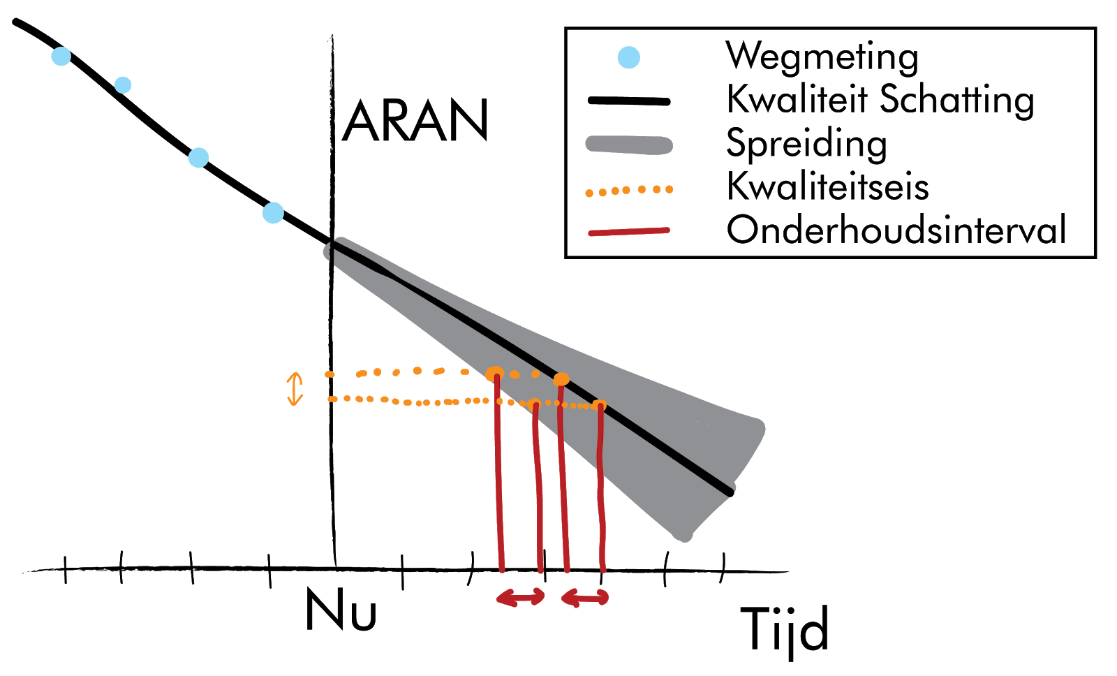
Figure 1: Simplified ARAN prediction. ARAN measures lateral unevenness (track formation) and longitudinal unevenness (bumps). Based on measurements (blue dots) a prediction (black line) is made with an uncertainty (grey area). Road quality thresholds (yellow lines) determine the period in which maintenance has to be performed (red lines).
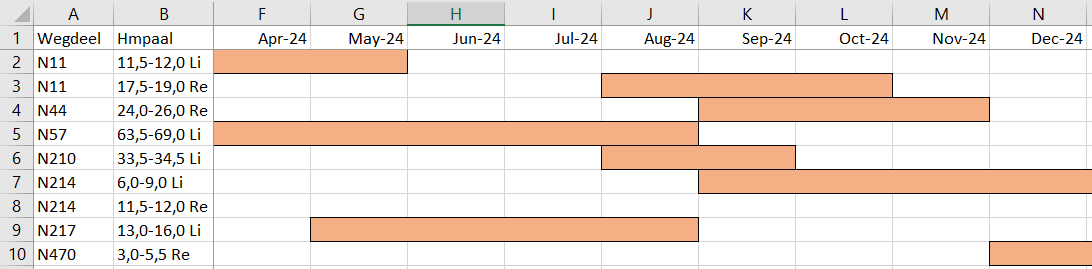
Figure 2: An example of the planner interface. The possible maintenance periods for each road are exported to Excel to offer an overview of the planning possibilities. The user can then tweak taking into account constraints such as closures of nearby roads.
Figures 1 and 2 can be seen as additional displays in the cockpit of road maintenance planners of the Province such that they can have improved control on road maintenance. The planners can therefore make their decisions more effectively and use their time more efficiently.
After the proposal we were invited for the pitching round after which we found ourselves to be the lucky winners!
The domain
A predictive model for road quality sounds great but is still a very abstract concept. It leads to questions such as: What is a road? What is road quality? What values are we trying to predict? When does a road need to be maintained? What kind of deterioration processes are there? Therefore, our first step was to understand the domain of road quality by consulting literature and domain experts from the Province to make these abstract concepts more concrete.
On roads
A road, in our case provincial N-roads, has been built at a certain time (year) and has one or more top-layers and an associated depth (asphalt types), one or more foundations and an associated depth (such as clinkers or grind) and an underlying soil type (such as sand). These parameters can be seen as the initial, structural conditions of the road. Based on literature and the expertise of domain experts, we make the assumption that at construction the road quality is highest and will degrade until maintenance is performed. After this, road quality will follow a sawtooth pattern with peaks caused by maintenance being performed, which decrease in height over time as can be seen in Figure 3.
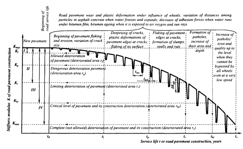
Figure 3: Sawtooth pattern of road quality (Regularities of defect development in the asphalt concrete road pavements, Sivilevičius & Pektevičius, 2002)
Road quality indices
Different aspects of roads can be seen as quality indices of which the most important ones are:
- Longitudinal and lateral unevenness (indicating bumpy roads and track formation)
- Skid resistance (indicating the grip of a tire)
- Fraying (indicating the quality of the asphalt)
- Cracks (indicating the quality of the asphalt)
- Falling weight deflection (indicating the quality of the foundation)
- Depth of the different layers (indicating the quality of the foundation)
There are standardized methods, such as ARAN, drilling and VWI (visual road inspection), to measure these parameters and the Province of Zuid-Holland appoints multiple parties to perform these measurements every so many years. The Province has started collecting these measurements around 2004 and they form the historical data on which a model can be trained.
Features affecting road quality
From literature and our discussions with domain experts, it became clear that there are two important factors affecting the degradation of road quality: usage and climate. It is often a combination between these factors that results in interesting features. For example, high temperatures result in higher elasticity of the asphalt. Combined with heavy loads this results in both increased track formation and reduced skid resistance (Factors influencing track formation in asphalts, Ambrus, 1995), (Prediction of Rutting Formation in Asphalt Concrete Pavement, Haritonovs, 2010)
Furthermore, rain before frost can result in plastic deformation due to the expansion of ice: water enters the asphalt after which the frost sets in and the water within the asphalt expands resulting in cracks in the asphalt (Regularities of defect development in the asphalt concrete road pavements, Sivilevičius & Pektevičius, 2002)
By taking these degradation features into account a predictive model will be closer to reality, and as a result proof more useful.
Approach
Now the idea behind the predictive model that we are trying to build starts to take shape: Roads have initial structural conditions such as their construction year and foundation and multiple quality indices which are measured every so many years. Furthermore, there are features such as heavy loads and high temperatures and frost combined with rainfall which degrade these quality indexes. A predictive model could try to predict these quality indices based on initial conditions, historistic data and continuous data corresponding with features affecting the road quality.
To create such a model we have proposed three milestones, such as can be seen in Figure 4. Firstly, in milestone 1 (data engineering), data coming from different sources (Province, KNMI, external sources), in different formats (ESRI shapefiles, XML, csv) and with different qualities, has to be gathered, understood, filtered and preprocessed. The major challenge here is to decide on the scope of a predictive model, i.e. choose a way in which to discretise a road into smaller objects and then to connect these smaller objects with the data. The result of this milestone is a workable and representative dataset.
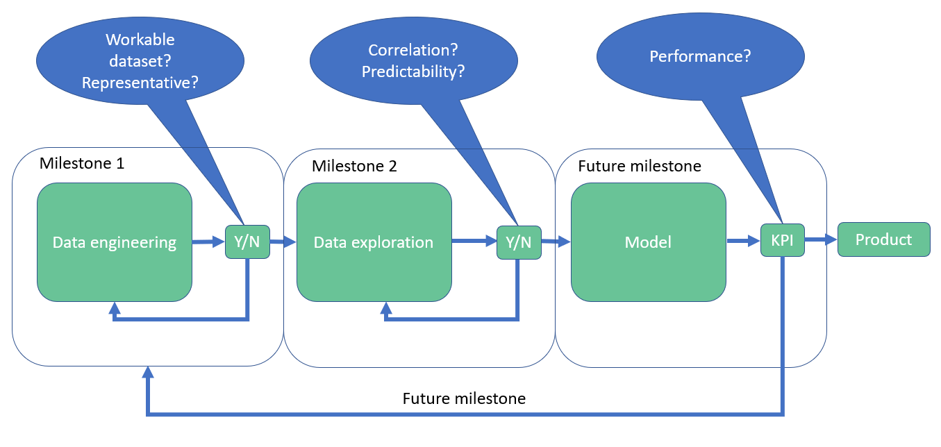
Figure 4: Proposed and agreed milestones to develop a predictive model.
Secondly, in milestone 2 (data exploration) analysis is performed on this dataset to determine correlations, important features and as a result the feasibility of a predictive model. Depending on the strength of these correlations a decision will be made about future milestones.
After this milestone a decision will be made about the continuation based upon the degree of correlation and the feasibility of a model with the current dataset. Some of the possible continuations are: 1. create a model (correlation and enough data), 2. iterate over data engineering and data exploration (weak correlation / not enough data), 3. a thorough analysis of why currently a model can’t be build and what has to change to make a model possible (no correlation / correlation but the wrong data / …).
Milestone 1: Data engineering
Milestone 1 consists of a couple of requirements:
- Decide which roads to use as input
- Decide how to discretize these roads to allow for a predictive model
- Gather available data on these roads
- Gather data concerning the features impacting road quality
- Connect the data to the decided road discretization
Firstly, the Province decided on the roads to take as input: N223a N215a N207a N468a
Secondly, so-called beheerobjecten were chosen together with the Province to serve as the discretized parts of a road. The Province has classified its roads in trajecten (N223), traject parts (N223/A and N223/B) and beheerobjecten (N223/A/1/10). An example of a beheerobject as drawn in a geographical information system (GIS) can be seen in Figure 5.
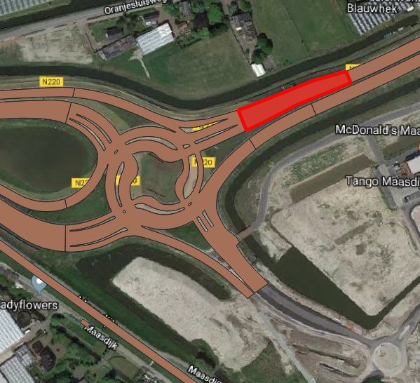
Figure 5: Part of the beheerobjecten within the trajectdeel N223/A, the selected beheerobject (red) is N223/A/10/120.
The next step was to connect these beheerobjecten with the available datasources. This turned out to be quite a challenge due to the poor data quality: all measurements were associated with some sort of geospatial reference (GPS, rijksdriehoekstelsel, hectometering) and all of these references contained major errors. Therefore, we developed an algorithm to correct for these errors of which the results can be seen in Figure 6.
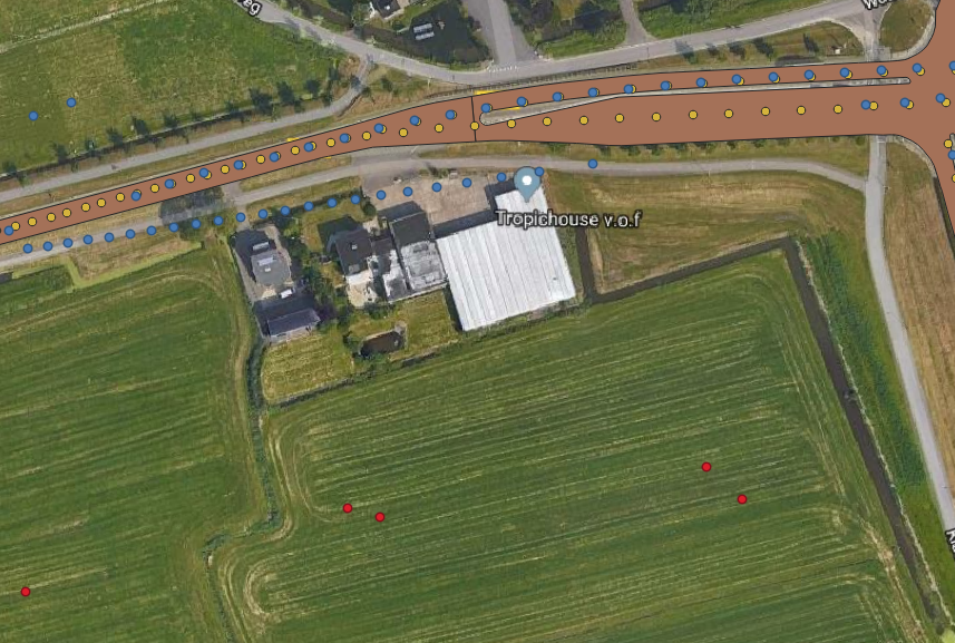
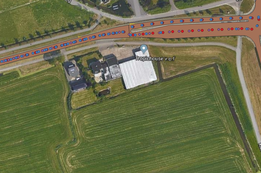
Figure 6: Top: geospatial references before correction. Bottom: geospatial references after correction. The attentive reader will notice that there are more red measurements (ARAN 2017) in the bottom image than visible in the top image. These measurements have an even higher error than the ones visible in the top picture and therefore fall outside the picture.
Using this algorithm we managed to correct bad measurements while throwing away between 2-3% of the data points which we deemed unfixable. To put this in perspective, an earlier attempt to correct for these measurements resulted in 10% of the data points being thrown away and was more likely to perform bad corrections due to its hardcoded nature, although this is something we cannot validate. With these data points, we now have the initial structural conditions and historic measurements associated with beheerobjecten.
In parallel, we gathered data associated with road usage coming from induction loops under the roads. The Province has 255 of these loops and these measure the length and speed of a passing vehicle by analysing the induced current, based on these lengths vehicles can be classified into categories such as cars and trucks. On this data preprocessing had to be performed to result in output such as can be seen in Figure 7.
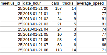
Figure 7: Processed measurements from meetlus 25. For each hour the passing cars, trucks and average speed are determined.
Furthermore, these measurements have to be matched to beheerobjecten which requires geospatial processing of which the result can be seen in Figure 8. This processing uses a distribution model of induction loops to roads provided by the Province.
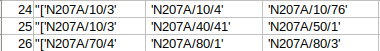
Figure 8: Induction loops matched to beheerobjecten.
Parallel we gathered, preprocessed and matched FloatingCarData, which is sensory data collected via phones and in car navigation system, to have a more precise average speed throughout the road network.
We also looked into the possibility to include the Weigh in Motion loops, which measure the total weight travelling over the road but since there are only 2 of these loops present in the roads of the Province they are not taken into account for now. It could be interesting to add these later on to determine the correlation between length and weight to have a more accurate load distribution throughout the road network.
Lastly, we gathered open climate data of the KNMI: hourly rain measurements via a 1×1 km2 radar grid and hourly temperature and sunhours via the KNMI weather stations.
An overview of the gathered data can be seen in Figure 9. Firstly, the Province provides us with historical road quality measurements and initial structural conditions. Secondly, the Province provides us with induction loop data and FloatingCarData. Lastly, we retrieve climate data via the KNMI in a raingrid and measurements associated with weather stations. All these measurements require preprocessing and geospatial matching.
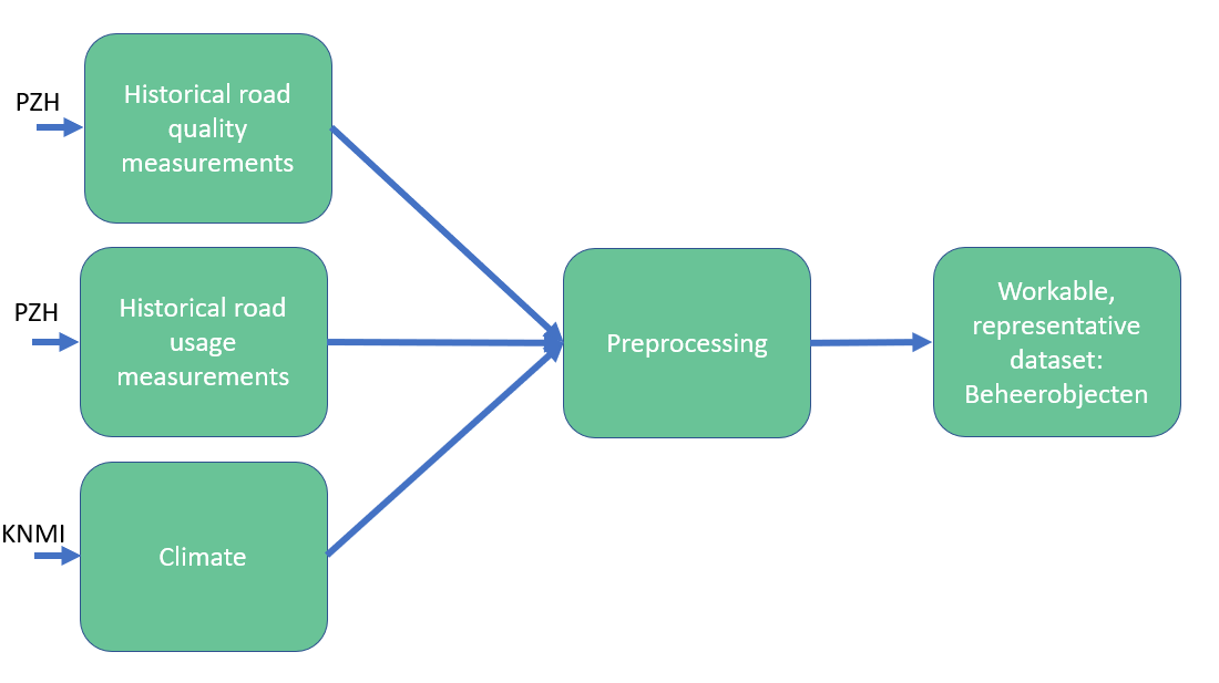
Figure 9: Overview of the gathered data.
On Wednesday the 14th of August we presented milestone 1, in which we showed the workable, representative dataset to the Province. Already, with the availability of this dataset, more insight is possible into the status of roads. Furthermore, a very important result of this milestone is an advice, followed by the Province, to put stricter requirements on the localisation associated with measurements for future tenders to external measurement parties.
After this meeting, we agreed upon the start of milestone 2, data exploration, which we are currently embarking upon. We will keep you updated through our website!