
0) Introduction
Imagine that we are coding a very simple software to sort a list of elements. We finish writing our application in whatever programming language we feel most comfortable with, and execute it on a randomly generated list of N numbers, counting the time it takes to execute it, and getting a result of 100ms.
We try on different lists of size N and get an average result similar to the 1st one: 100ms. Now we double the size of our list to 2N, and do the same. When we get the results however, it isn't taking an average of 200ms (double the previous time), but more, an average of 250ms. Moreover, we double again the number of items to 4N, and the time is not double the previous one, which would be 500ms, but rather 600ms.
What is happening here?
To understand it we need to know what Computational Complexity is all about, and take a look at its associated Big O notation. In this post, we will clearly explain these concepts, see some examples of Computational Complexity and Big O notation, and get some some insights into why it is important to consider the complexity of our algorithms when coding.
To end, we will also mention why Computational Complexity is relevant in the world of Machine Learning and Big Data.
TLDR:
- What is Computational Complexity?
- The Big O Notation Explained
- Avoid the Exponentials
- Computational Complexity in Machine Learning
- Conclusion and further Resources
1) What is Computational Complexity?
When we code a program to do a certain task, the underlying logic of our programming (the structure and flow of the code, the functions that we use, etc…), makes our code have to run a specific number of operations.
These operations, in turn, take their time, so generally the more operations that our programs executes, the higher the time it will take for it to run.
Computational Complexity, in one of its forms, refers to the relationship between the increase in the time it takes an algorithm or program to run, and the increase in the input size of that algorithm or program. An example of this relationship is exactly what we saw in the example illustrated at the beginning of this post.
This kind of Complexity is known as Time Complexity, and we calculate it considering the time it takes to run our algorithms with regards to the input size. It is important to highlight this, because Space or Memory Complexity (which is the amount of physical space or memory that algorithms take up in our computers memory, another possible bottleneck) also exists, but in this article we will be speaking about Computational Complexity in terms of time.
Input size, however, is not the only characteristic of our data that can influence the operations and therefore the time it takes an algorithm to run: the actual data itself matters too. Imagine the sorting algorithm we spoke about in the introduction. If the data that we feed it is already sorted, it will probably take less than if the data is in a completely random order.
Because of this, when speaking about time complexity we can have 3 different perspectives:
- Best case scenario: when the information in the input size makes it so that the algorithm requieres the minimum number of steps to execute and reach its goals.
- Average case scenario: refers to the average number of operations required for input of the given size.
- Worst case scenario: refers to the maximum number of operations needed to carry out a task given an input size.
The worst case scenario is generally the one we should consider and try to improve, as from there there is an established threshold which can be used as a reference.
Lets see a couple of examples of complexity in sorting algorithms to make it all clearer. First, we will evaluate the complexity of a Selection Sort sorting algorithm, seeing how as we increase the input size, the time it takes to run it increases in a non-linear manner.
The code to sort an array using this algorithm is the following:
def selection_sort_func(array):
    """
    Selection sort algorithm to
    sort a given array of integers

    :param array: input array to the algorithm
    :return: array: array sorted after process
    """

    # Parametrize the length of the array
    n = len(array)
    # Find the minimum element in remaining array
    for i in range(n):
        min_index = i
        for j in range(i+1, n):
            if array[min_index] > array[j]:
                min_index = j

        # Swap the found minimum element with the first element
        array[i], array[min_index] = array[min_index], array[i]

    return array
In it, we can see that selection sort uses two loops: an outer loop to run through every item of the array, and an inner loop to run through the items of the array that are ahead of the one from the outer loop.
This outer loop runs n -1 times and does two operations per run, one assignment (min_index = i) and one swap (array[i], array[min_index] = array[min_index], array[i]), resulting in a total of 2n-2 operations.
The inner loop runs for n-1 times, then for n-2, then for n-3 and so on. This sun of all these runs can be expressed as the following series:
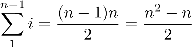
In the worst case (the scenario which we have to consider which we saw before) the if condition is always met, so this inner loop executes 2 operations, a comparison (if array[min_index] > array[j]) and an assignment (min_index = j), resulting in a total of n²- n operations.
In total, taking into account the inner and outer loop, the algorithm costs 2n-2 operations for the outer loop plus n²- n for the inner loop, resulting in a total number of operations and therefore a time complexity of T(n) = n²+ n -2.
Seeing this formula, lets evaluate what happens when we go from lets say 100 items in the list, to 200.
T(100) = 10000+ 100 -2 = 10098
T(200) = 40000+ 200 -2 = 40198
T(200)/T(100) = 40198/10098 = 3.98
It 3.98 times more to sort 200 items than to sort 100 items! Also, see how this number is very close to 4? As we increase the input size we are compering, this gets closer and closer to 4, meaning it would take 4 times as long to sort 2 million items than to sort 1 million items.
Lets check this in code. The following script uses the previously shown selection_sort_func function to sort the elements of two randomly created integer arrays, one with size 1000 and one with size 2000.
import numpy as np
import time
from sorting_algs import selection_sort
max_value = 20000
input_size = 1000
random_array = np.random.randint(low=0, high=max_value, size=input_size)

start = time.time()
sorted_array = selection_sort.selection_sort_func(random_array)
end = time.time()

print(f"For an input of size {input_size} the algorithm took {end - start} ms to execute")

input_size = 2000
random_array = np.random.randint(low=0, high=max_value, size=input_size)

start = time.time()
sorted_array = selection_sort.selection_sort_func(random_array)
end = time.time()

print(f"For an input of size {input_size} the algorithm took {end - start} ms to execute")
If we run this script the output is the following:
For an input of size 1000 the algorithm took 0.1246945 ms to execute.
For an input of size 2000 the algorithm took 0.5066458 ms to execute.
See how much longer it takes to sort the list when it is twice as long? To make this more fair, we should run the algorithms multiple times on each input size, and average the results, but you get the idea, right?
Most times, instead of considering the whole equation of the complexity (T(n) = n²+ n -2) what we do is keep the highest order term, as it usually dominates the rest, specially as the input size n grows.
With all this previous information, we would say that the Computational Complexity (time wise) of the Selection Sort algorithm is of T(n) = n².
The following figure shows the comparison between the growth in different types of complexities as the input size increases.
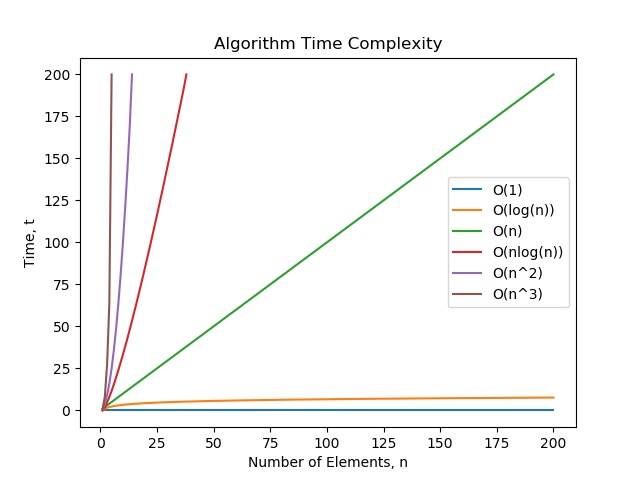
There is a little spoiler about Big O notation on the legend, but just stay with me for a second and think of those of T(1), T(log(n)), and so on for the moment.
We can see some interesting stuff here:
- T(1) means that the computational complexity is constant: it does not depend on the input size. If you take a look at the most common operations in Python and their time complexity (here), you can see that operations such as appending an element at the end of a list has this kind of complexity.
- For large input sizes, up to linear T(n), the time increases in a controlled manner.
- For linear and above (all the lines to the left of the green diagonal), time complexity skyrockets as we increase the input size.
- Cubic and squared complexities seem to rise incredibly high, but there are other evil complexities which we will explore in the following sections that are much, much worse: the exponential and the factorial.
Other sorting algorithms like the famous Bubble Sort, have the same time complexity than Selection Sort, leading to similar increases in the execution time as we increase the sample size. The code for bubble sort can be found here:
def bubble_sort_func(array):
    """
    Bubble sort algorithm to
    sort a given array of integers
    :param array: input array to the algorithm
    :return: array: array sorted after process
    """

    # Calculate the length of the array
    n = len(array)
    # Traverse through all array elements
    for i in range(n - 1):
        # Last i elements are already in place
        for j in range(0, n - i - 1):
            # traverse the array from 0 to n-i-1
            # Swap if the element found is greater
            # than the next element
            if array[j] > array[j + 1]:
                array[j], array[j + 1] = array[j + 1], array[j]

    return array
If we execute both sorting algorithms on the same arrays of size 1000 and 2000, we get the following results, which are very similar, with slightly better performance for the selection sort.
Selection Sort
For an input of size 1000 the algorithm took 0.130644 ms to execute
For an input of size 2000 the algorithm took 0.517642 ms to execute
Bubble Sort
For an input of size 1000 the algorithm took 0.136633 ms to execute
For an input of size 2000 the algorithm took 0.551555 ms to execute
Lastly, lets check out Quicksort, before we move on to explain what Big O Notation is, so that you can see how a different and better time complexity can have a huge impact on the performance of our algorithms.
Quicksort is a recursive sorting algorithm that has computational complexity of T(n) = nlog(n) on average, so for small input sizes it should give similar or even slightly poorer results than Selection Sort or Bubble Sort, but for bigger inputs the difference should be very noticeable.
The code for the Quicksort algorithm is the following: as you can see we have to implement a helper function to partition the array. You can learn all about Quicksort here.
import numpy as np

def partition(array, low, high):
    """
    Function that takes the last element as pivot
    places the pivot element at is correct position
    in the sorted array, and places all smaller elements
    to the left, and greater to the right

    :param array: array to sort
    :param low: smaller element
    :param high: bigger element
    :return: index where partition must occur
    """
    # index of smaller element
    i = (low -1)
    # Calculate pivot at random
    pivot_index = np.random.randint(low=0, high=len(array))
    pivot = array[pivot_index]

    for j in range(low, high):

        # If current element is smaller than or
        # equal to pivot
        if array[j] <= pivot:

            # increment index of smaller element
            i = i+ 1
            array[i], array[j] = array[j], array[i]

    array[i + 1], array[high] = array[high], array[i + 1]
    return (i + 1)


def quick_sort_func(array, low, high):
    """
    function that implements the quicksort
    sorting algorithm
    :param array: array to sort
    :return:
    """
    if len(array) == 1:
        return array
    if low < high:
        # pi is partitioning index, arr[p] is now
        # at right place
        pi = partition(array, low, high)

        # Separately sort elements before
        # partition and after partition
        quick_sort_func(array, low, pi - 1)
        quick_sort_func(array, pi + 1, high)
Lets see what results we get for arrays of input sizes 1000 and 2000 like before:
Selection Sort
For an input of size 1000 the algorithm took 0.1226947 ms to execute
For an input of size 2000 the algorithm took 0.4907164 ms to execute
Bubble Sort
For an input of size 1000 the algorithm took 0.1326408 ms to execute
For an input of size 2000 the algorithm took 0.5295898 ms to execute
Quick Sort
For an input of size 1000 the algorithm took 0.0169501 ms to execute
For an input of size 2000 the algorithm took 0.0388991 ms to execute
We can see how for size 1000, it is slightly worse than the other two, but for double that, size 2000, it has better performance, making it evident that it scales better with size than Bubble Sort and Selection Sort. This difference is even more dramatic if we increase the input size even more. Lets see it!
Check out what happens when we use 5000 and 10000 as the input sizes of our arrays:
Selection Sort
For an input of size 5000 the algorithm took 3.0628ms to execute
For an input of size 10000 the algorithm took 12.8446ms to execute
Bubble Sort
For an input of size 5000 the algorithm took 3.4507ms to execute
For an input of size 10000 the algorithm took 13.9834ms to execute
Quick Sort
For an input of size 5000 the algorithm took 0.16954ms to execute
For an input of size 10000 the algorithm took 0.42389ms to execute
Amazing differences right? In these kind of problems where size definitely matters, picking the right algorithms is very very important.
I hope these examples have made it crystal clear why it is important to consider the complexity of our algorithms when building real applications that use considerable amounts of data.
In the next section we will clarify how this is all related to Big O Notation, what Big O complexity is, and how it all builds up into an awesome analysis framework to think about when developing software.
Lets get to it!
2) The Big O Notation Explained
As we saw in the previous section, one of the most relevant issues we have to consider when evaluating a specific algorithm for an application is how it scales or grows: how its performance is affected by variations in the input size.
This concept of growth is what Big O Notation quantifies. It is a notation that specifies the most dominant term in an algorithms Time Complexity (worst case scenario time complexity), and therefore the way its execution time is affected by changing the input size.
Also known as Big Oh or Big Omega notation, it is the standard information to look up when carrying out a complexity analysis for an algorithm or application. By looking up the Big O notation complexities of the different operations carried out, we can infer the Time Complexity of the whole system, and have an idea of how well our application would scale with more data.
Having Big O notation in mind can help us choose the best pieces of code to base our software on, helping us build more efficient programs, and leading us towards good coding practices like trying to avoid using an excessive number of loops, or nested pieces of code that increase complexity dramatically.
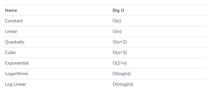
The following are the most common Big O Notations:
For most programming languages there exists documentation about the Time complexity of the operations of the most common functions like inserting or removing elements from a list, looking up values in dictionaries, etc…which we should consider when we are building our software.
The following shows the time complexity for the most common operations used on Python lists. You can find the Time Complexity python documentation here.
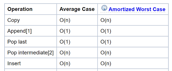
From this table we can see that appending an item to a list has a constant time complexity as we saw before: all you have to do is put an element at the end of it, without having to iterate through all its elements.
Inserting an element on the list on the other hand, puts a new item on an specific index, so it does have to iterate through the list, and in the worst case it has to go through all of it until it reaches the desired index.
Big O Notation is super useful when designing software, as it allows us to pick the best options in almost every aspect we should evaluate.
It is very relevant when storing data too, as certain data formats take a longer time to update and retrieve information from than others. If we want to build applications that work in real time (RT), then time complexity is something we always have to consider, as we might have to ditch the confortable and well known tabular storage format in change for a higher performance.
Now that we know what Big O is, and why is important, lets see some of the most undesirable time complexities, and what kind of operations can lead to them.
3) Avoid the Exponentials
Having understood what Big O Notation is, there are two main complexities which we should always try to avoid, as if our applications have operations with these kind of complexities, they will scale very very poorly, even to moderate amounts of data.
These are the infamous exponential(2^n), and even worse, the factorial (2!). Algorithms with these kind of complexities grow so fast, that they can only be used for certain types of inputs, and even then requiere a very large sum of time to execute.
The following figure compares the growth of some the most common complexities with the input size. As we can see, the exponential has a much larger growth than the quadratic or squared complexity ( T(n) = n²) that we saw before, and that one was already a fast growing one.

Because of this, it is almost inviable to execute programs that have exponential or even worse, factorial complexities. In these cases, not even huge amounts of computing power will be enough, and the problem probably would have to be tackled in a different manner to avoid reaching insanely high execution times.
Some examples of problems with exponential complexities are:
- The Power Set problems: finding all the subsets on a set.
- Computing the Fibonacci sequence.
- Solving Travelling salesman problem using Dynamic programming.
Awesome, now that we know which kind of complexities we should avoid, lets end this post with a sweet pinch of one of our favourite pieces of cake of the Computer Science world: Machine Learning and Data Science.
4) Computational Complexity in Machine Learning
As most of us know, Machine Learning is all about data. Possibly lots of data. Big Data. Because of this, special care has to be put when designing Machine Learning applications, as even simple pieces of software like formatting data, or merging tables, can take a very long time on the data with the size of that ML algorithms are trained with.
Even more, each machine learning model has its own characteristics (training procedure and prediction mechanisms), resulting in a certain time complexity. Depending on the amount of data that you have available at the moment of training, you should consider using one algorithm over another. Prediction time complexity should also be relevant if you plan on predicting at once on large batches of new data, or on working in real time.
Also, Machine Learning models have something particular to them: the complexity is not only a function of the input size n, but also of the number of features of our data d. Using these two parameters we should mindfully pick what models we ought to use, as for high values of these parameters, some models will take outrageous amounts of time to train, even on powerful GPUs.
The following table shows the training time complexities for some of the most popular Machine Learning models:
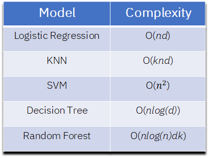
As we can see, Logistic Regression has a linear growth with relationship to the number of data points and features. Decision Trees have a linear growth with relationship to the data size and logarithmic with relationship to the number of features. In Random forest and K-Nearest Neighbour, the k refers to the number of trees in the forest in the first case, and to the number of neighbours in the second.
Also from the table we can point out that SVMs have a quadratic complexity with relationship to the input size n, which means that they should not probably be used to train on very big amounts of data, however, the number of features of this data is not so relevant. This is because the increase in the time complexity with regards to the input size dominates the growth so much that the number of features is almost irrelevant to the training time complexity of the model.
This means that they work well for small, complex data sets, that is, where the number of training samples is not very large, but that can have a lot of features (see Geron, ‘Hands on Machine Learning with Scikit-Learn, Tensorflow, and Keras’, Chapter 5: Support Vector Machines).
Knowing about the complexity of our algorithms as a Data Scientist or Machine Learning engineers can help us make decision aside from technical ones: If we train a Logistic Regression classifier on some data, we can go grab a coffee, come back, and its probably done.
If we choose to pick an SVM, or an Artificial Neural Network (not on the table, but also an family of models that takes a long time to train), we can probably go for a walk, have lunch, read a bit, work on some other project, go home, have dinner, go to sleep, wake up, go back to work to check how our algorithm is doing, and it will still probably be training.
If we have deadlines whatsoever that we must accomplish in an specific amount of time, it is probably a good idea to get a basic model that runs fast, even tune that model to extract from it its best possible performance, and avoid using models that take a lot of time to train, as tuning these models, with even a small hyper-parameter grid search can take a long while.
Awesome! I hope that with this last little bit, you have managed to see other fields of Computer Science where Complexity is very relevant, and specifically how it should be something that is always in our toolbox for decision making in the realm of software.
5) Conclusion and Additional Resources
In this post we have seen what Computational Complexity is, how it is expressed with the Big O Notation, and why it is so important to consider it when building software applications that have an input that can grow or scale.
The quote by Ada Lovelace that this article started with states it very clearly: when building software applications we must design them in the way which leads to the most efficient code and least calculations, and to do that, we must know about Complexity and the Big O Notation.
Here are some additional resources in case you want to go deeper into any of the topics covered in this article, like sorting algorithms, more information about complexity, or how Machine Learning is affected by it.
- The most well known sorting algorithms video.
- Sorting algorithms and Big O Notation video.
- Python operations Time Complexity.
- Rescursive functions — GeeksforGeeks.
- Space Complexity Wiki.
Additionally, you can find all the code used for the examples in this article on my GitHub, on the following repo. For further resources on Machine Learning, Python Programming and computer science, check out How to Learn Machine Learning.