Distance Metrics for Machine Learning

0) Introduction

 ‘Whats the distance between Madrid and London?’

‘ How alike are Tom and Lucas?’

‘Which song should my software recommend?’

These questions might all seem to search for very different insights. However, when answered from the realm of data, they all have one thing in common: they can be partially or completely answered using the same family of metrics: Distance Metrics. 

The goal of this post is to explain what distance metrics in the Machine Learning world are, why they are relevant, and how they affect our algorithms and models.

We will cover the general concepts and ideas, and then see the most used distance metrics and learn how to implement them in Python to get a better understanding. 

Everything will be delightfully explained, so sit back, relax, and enjoy. 

Lets get to it. 

TLDR;
1. What are Distance Metrics?
2. Why do we need Distance Metrics in Machine Learning?
3. Euclidean Distance
4. Manhattan Distance
5. Minkowski Distance
6. Hamming Distance
7. Tips and Tricks when using Distance Metrics
8. Conclusion and further Resources

1) What are Distance Metrics?

When assessing how similar two data points or observations are, we need to calculate some sort of metric to be able to compare them. Distance Metrics allow us to numerically quantify how similar two points are by calculating the distance in between them.

When the calculation of a distance metric leads to a small quantity, it means that the two points are similar, when it is big, they are different. Easy right?

You could think, alright, cool. But whats with all the fuss? The distance in between to things is always the same. What is all the big deal? 

The answer my friend, is that it is not always as straightforward as you might intuitively think. Consider Google Maps for example. 

If we want to go from Times Square to the Rockefeller Center, it tells us to follow the blue dotted line: going down 7th Av, then turning right at W 47th St, crossing a passage in between 7th and 6ths Av, and then turning right again at W 48th to finally glance our destination. This guidance follows the logic behaviour that stops us from going in a straight line and crushing our head into a wall. 

The distance we have to travel following the blue dotted line (called Manhattan Distance, which we will see later) and the distance along the straight red line (Euclidean distance) are different. 

What does this mean? It means that there are different ways to measure distances, which lead to different results. Why is this relevant to us, Machine Learning and Data Science knights? Lets see why 🧐.

2) Why do we need Distance Metrics in Machine Learning?

The reason that we should care about this is because these distance metrics are used in many of our favourite algorithms like K-Nearest Neighbours Classification algorithm, K-Means Clustering algorithm, or Self-Organising Maps (SOM). Some Kernel Algorithms like Support Vector Machines use calculations that can be considered as ‘distance calculations’ too. 

Because of this, it is important to understand what the logic behind each distance metric to know when we should use one versus another, as this can have a big impact in the results of these previous algorithms or models. 

Depending on the kind of data we have, the algorithm that we are using, and the intuition behind it, we might want to use one distance metric over another one, so it is good to have at least a basic understanding on what each metric represents. 

Now that we know that Distance Metrics are, and why they are so relevant, lets take a look at the most widely used metrics. 

3) Euclidean Distance

Euclidean Distance is the de-facto distance metric. Remember the famous Pythagoras theorem we all learn in high school? 

It goes like this: 

“In a right-angled triangle, the square of the hypotenuse side is equal to the sum of squares of the other two sides”

Euclidean distance is calculated using this theorem, and it gives us the ‘straight line’ distance we saw in the Google Maps example. It tells us how far away point A is from point B if we follow a straight line. 

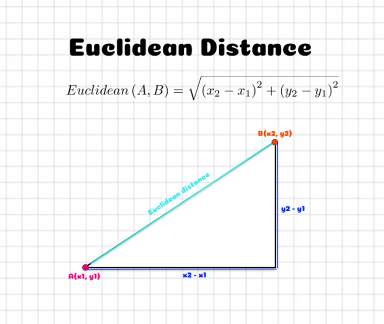
The previous figure shows how this is translated into a 2D plane. If we have two points [A(x1, y1)] and [B(x2, y2)], the Euclidean distance in between them is the square root of the sum of the squared differences in between X coordinates and the Y coordinates (which are the sizes of the sides of the right-angle triangle).

Because of this squaring the Euclidean Distance is always positive. 

What does this have to do with Machine Learning? It just looks like Geometry. 

Wait.

Imagine that now A and B are two observations from our data set, with x1, and y1 being the two features of observation A, and x2, and y2 being the two features of observation B. Now, calculating the Euclidean Distance would tell us how similar A and B are, and we could use this similarity to make predictions or group our observations. Awesome right?

In the Machine Learning world the Euclidean Distance is also known as the L2 distance, as it is calculated similarly to the L2 norm. 

In the previous example we have defined the Euclidean Distance for two dimensions (observations with two features) for the ease of visualisation, however, it is easily expandable to N-dimensions. The formula is the following: 

In this formula A and B are our observations, and fai and fbi are the ith feature of observation A and observation B respectively. 

So when should we use the Euclidean Distance? As mentioned earlier, this is usually the default distance metric used by most algorithms and it generally gives good results. Conceptually, it should be used whenever we are comparing observations which features are continuous, numeric variables like height, weight, or salaries for example. 

Lets see the code for implementing the Euclidean Distance in Python:

import numpy as np

#Function to calculate the Euclidean Distance between two points
def euclidean(a,b)->float:
    distance = 0
    for index, feature in enumerate(a):
        d =(feature - b[index])**2
        distance = distance + d
        
    return np.sqrt(distance)

This code calculates the Euclidean distance between two points a and b. It is not necessary to implement this function to calculate it tough, as libraries like numpy or scipy have their own implementations of the metric calculation:

from scipy.spatial import distance

# Our observations
a = np.array((1.1, 2.2, 3.3))
b = np.array((4.4, 5.5, 6.6))

numpy_dist = np.linalg.norm(a-b)
function_dist = euclidean(a,b)
scipy_dist = distance.euclidean(a, b)

All these calculations lead to the same result, 5.715, which would be the Euclidean Distance between our observations a and b. 

Awesome, now we have seen the Euclidean Distance, lets carry on two our second distance metric: The Manhattan Distance 🌃.

4) Manhattan Distance

We’ve covered the red, straight-line example from the Google Maps example. But what about the Blue Dotted route? We mentioned earlier that this was called The Manhattan Distance. Whats the intuition behind it? 

The Manhattan Distance, also know as L1 Distance or City Block distance calculates the sum of the absolute values of the difference of the coordinates of the two points, rather than squaring them and then calculating the squared root of the sum. This means that mathematically it has a less desirable formulation for Machine Learning problems (absolute values mess with derivatives) than the Euclidean Distance.

The following Figure shows the intuition Behind it. 

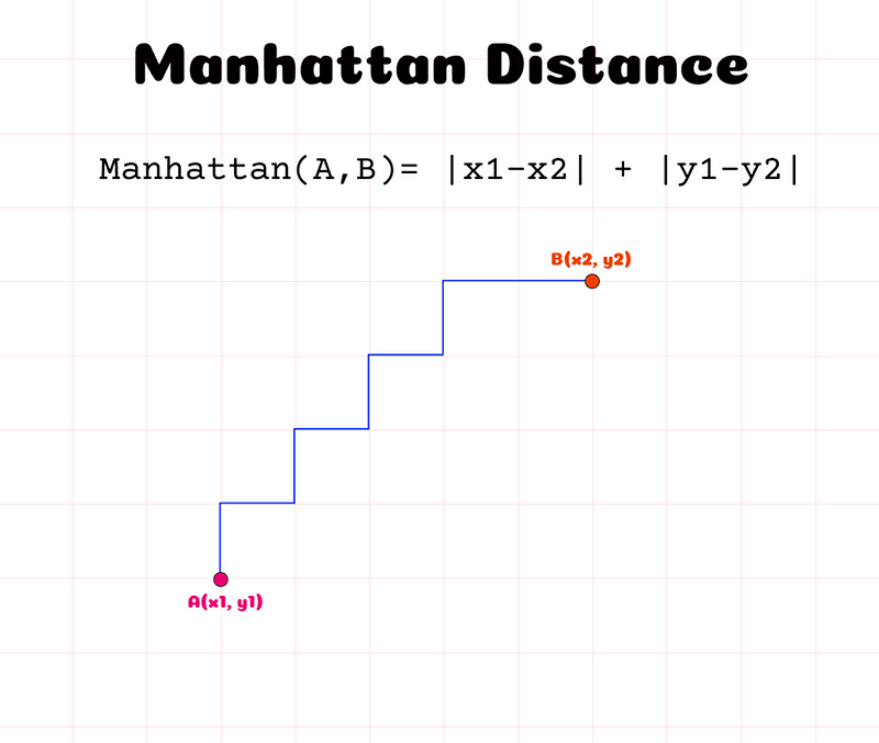
The Manhattan distance calculates how many squares in a grid (or blocks in a city like Manhattan, since where the name comes from) we would have to go through to get from point A to point B. Instead of taking the straight line like in the Euclidean Distance, we ‘walk’ through available, pre-defined paths. 

As in the example with the Euclidean Distance, this previous illustration represents the 2 dimensional calculation, but it is easy to generalise it to N dimensions using the generic Manhattan Distance formula: 

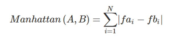
The Manhattan distance is useful when our observations have their features distributed along a grid, like in chess or city blocks. What this means is that it makes sense to use the Manhattan distance when the features of our observations are entire integers (1,2,3,4…) with no decimal parts. The Manhattan Distance always returns a positive integer.

The following code allows us to calculate the Manhattan Distance in Python between 2 data points: 

import numpy as np

#Function to calculate the Manhattan Distance between two points
def manhattan(a,b)->int:
    distance = 0
    for index, feature in enumerate(a):
        d = np.abs(feature - b[index])
        distance = distance + d
        
    return distance

We’ve briefly spoken about when to choose Euclidean vs Manhattan and vice versa, however, our data rarely has all the features either continuous or integer like. Because of this if we have time, it might be best to try both metrics and see which one yields the best results. 

Instead of having to change from one distance metric to another in our pipelines, there is generic distance metric that through a hyper-parameter can calculate either the Manhattan Distance(L1 distance), Euclidean Distance (L2 distance), or higher value norm distances (L3, L4…). 

By changing a hyper-parameter of this generic distance metric, we can easily search for the best distance metric for our purpose. We are speaking about the Minkowski Distance. Lets check it out 👀.

5) Minkowski Distance

As mentioned earlier, the Minkowski distance is a generic distance metric that follows a pattern which allows us to play with a hyper-parameter in order to calculate the previous two distance metrics (Manhattan distance and Euclidean Distance) or higher norm metrics. It is basically a generalization of both the Euclidean distance and the Manhattan distance. 

The following is the formula for the Minkowski Distance between points A and B:

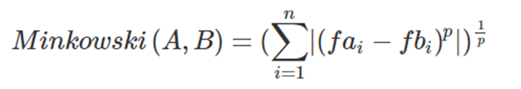
As we can see from this formula, it is through the parameter p that we can vary the distance norm that we are calculating. The Minkowski distance with p = 1 gives us the Manhattan distance, and with p = 2 we get the Euclidean distance. Also p = ∞ gives us the Chebychev Distance. 

p can also be given intermediate values between 1 and 2 (or any other integer number actually), which in the case of a decimal number between 1 and 2 (like 1.5 for example) provide a controlled balance between the Manhattan and the Euclidean distance. 

It is common to use Minkowski distance when implementing a machine learning algorithm that uses distance measures as it gives us control over the type of distance measure used for real-valued vectors via a hyper-parameter “p” that can be tuned. 

If you are implementing an algorithm that uses distance metrics and are not sure which one you should use, then using the Minkowski distance with a couple of different values of p (1, 2, and some intermediate values) and seeing which yields the best result, is a good approach for optimising your models. 

Now that we know what it is about, lets see the code to implement the Minkowski distance in Python. First we will do a self-made function to calculate the Minkowski distance in Python, and then we will use pre-made functions from available libraries. 

We start by importing the necessary libraries: 

# import libraries
import math
import numpy as np
from decimal import Decimal

Then, we implement a function to calculate the ‘p’ root of any value. This is needed to calculate the Minkowski distance: 

# Calculate the p root of a certain numeric value  
def p_root(value, root): 
      
    root_value = 1 / float(root) 
    return round (Decimal(value) **
             Decimal(root_value), 3)

Lastly, we define the function that calculates this generalised distance metric, which takes in two vectors or points and the value of the hyper-parameter p. 

# Function implementing the Minkowski distance
def minkowski_distance(x, y, p): 
      
    # pass the p_root function to calculate 
    # all the value of vector 
    return (p_root(sum(pow(abs(a-b), p) 
            for a, b in zip(x, y)), p))

Lets try it out! 🕵️‍♂️

# Our observations
a = np.array((1.1, 2.2, 3.3))
b = np.array((4.4, 5.5, 6.6))

# Calculate Manhattan Distance
p = 1
print("Manhattan Distance (p = 1)")
print(minkowski_distance(a, b, p))
# Calculate Euclidean Distance
p = 2
print("Euclidean Distance (p = 2)")
print(minkowski_distance(a, b, p)) 
# Calculate intermediate norm distance
p = 1.5
print("Intermediate norm Distance (p = 1.5)")
print(minkowski_distance(a, b, p))

First, we define our data points, and then we calculate the Minkowski distance using three different values of p: 1 (Manhattan Distance), 2 (Euclidean Distance) and 1.5 (Intermediate). 

This yields the following results:

Manhattan Distance (p = 1)
9.900
Euclidean Distance (p = 2)
5.716
Intermediate norm Distance (p = 1.5)
6.864

Awesome! Now that we know how to implement the Minkowski distance in Python from scratch, lets see how it can be done using Scipy. Scipy has the distance.minkowski function that directly does all the work for us: 

# Our observations
a = np.array((1.1, 2.2, 3.3))
b = np.array((4.4, 5.5, 6.6))

from scipy.spatial import distance
# Calculate Manhattan Distance
p = 1
print("Manhattan Distance (p = 1)")
print(distance.minkowski(a, b, p))
# Calculate Euclidean Distance
p = 2
print("Euclidean Distance (p = 2)")
print(distance.minkowski(a, b, p))
# Calculate intermediate norm distance
p = 1.5
print("Intermidiate norm Distance (p = 1.5)")
print(distance.minkowski(a, b, p))

This yields exactly the same results as our previous self-made function to implement the Minkowski distance (without rounding the decimals):

Manhattan Distance (p = 1)
9.899999999999999
Euclidean Distance (p = 2)
5.715767664977295
Intermediate norm Distance (p = 1.5)
6.864276616071283

Great, now that we have seen what the Minkowski distance is, what is p in the Minkowski distance, when to use the Minkowski distance, and how to use it, lets get to our final metric: The Hamming Distance. ⛓

6) Hamming Distance

The Hamming Distance is the last of the distance metrics that we will see today. This specific metric is useful when calculating the distance in between observations for which we have only binary features.

This means that the Hamming distance is best calculated when all of the features of our data take either 0 or 1 as a value. It is basically a metric used to compare binary strings (understanding for strings here a row of binary features). 

If we have a dataset that is composed of ‘dummy’ boolean features, then the Hamming Distance is probably the best to compute the similarity between two data points. It is easily calculated by counting the number of positions where the two binary strings have a different value.

Imagine we have a data set made up of customers of a Telecom company, and we want to cluster the users by how similar they are. This data set only has binary features like Gender_Woman, Status_Married, Age_from_18_to_32, and more of this kind that only take 0 or 1 as their posible values. 

When we want to calculate the similarity in between two different users to see if they go in the same cluster, we can easily compute the Hamming Distance by counting the number of features which have different values, like shown in the following figure. 

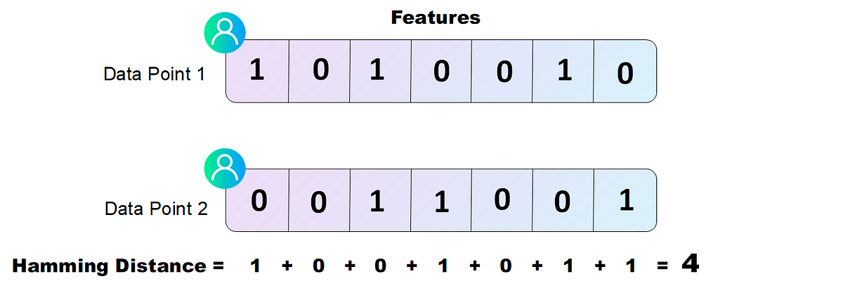
In practice, when speaking about binary strings the Hamming Distance can be computed by calculating the logical XOR in between the strings and summing the non zero values of the resulting string.

The following code shows how to do this, calculating the Hamming Distance in Python with the strings of the previous example using XOR:

# Our Data points with binary features
a = np.array((1, 0, 1, 0, 0, 1, 0))
b = np.array((0, 0, 1, 1,0 , 0, 1))

# Calculating the Hamming Distance using XOR and sum
hamming_distance = np.bitwise_xor(a,b).sum()
print(hamming_distance) # 4

This calculation gives us 4, exactly the same result as before. 

Most times the Hamming distance is normalised with the length of the strings we are comparing, to get a more general metric that is independent of such lengths. To do incorporate this to the previous code we just have to divide the result by the nº of features of our data: 

# Our Data points with binary features
a = np.array((1, 0, 1, 0, 0, 1, 0))
b = np.array((0, 0, 1, 1,0 , 0, 1))
# Calculating the Hamming Distance using XOR and sum
hamming_distance = np.bitwise_xor(a,b).sum()/len(a)
print(hamming_distance) # 0.571428

As always, Scipy gives us a way to do this all in one step with the distance.hamming function. Lets see how to calculate the Hamming Distance in Python using the library. 

# Our Data points with binary features
a = np.array((1, 0, 1, 0, 0, 1, 0))
b = np.array((0, 0, 1, 1,0 , 0, 1))
# Calculating the Hamming Distance Scipy
from scipy.spatial import distance

# Calculate Hamming Distance
print(distance.hamming(a,b)) # 0.5714

This gives us exactly the same result as before, 0.5714. 

Lastly, the Hamming Distance is used a lot in Natural Language Processing to calculate how two words or phrases of the same length differ:

‘Euclidean’ and ‘Manhattan’ both have 9 letters, so the Hamming distance in between them can be easily calculated by counting the number of different letters, which in this case is 7. 

7) Tips and tricks when using Distance Metrics

To end, lets note two or three quick tips and tricks about the calculation of distance metrics: 

• One obvious things that we have only mentioned in the last definition of the Hamming Distance is that these metrics can only be calculated if the two observations come from the same data set (have the same number of features). We can not calculate distance metrics between observations with different numbers or features, nor does it make sense to compute them if the nº of features is the same but the actual features vary. 
• When calculating distance metrics it is very useful to Normalise your features (bring them all to the same scale, preferably the 0–1 range) so that all the features weight the same in the calculation of the metric. Imagine we have 10 features, 9 which fall within the 1–10 value range, and one that goes from 0 to 1000000. If we don’t put them all on the same scale then this last feature which have a much higher weight on the calculation of the distance metric, which would be basically reduced to how much the observations differ on that specific feature value. 

8) Conclusion and further resources

Great! Now you know what distance metrics are, why they are relevant in the Machine Learning world, and you have learned how to implement the most important ones in Python. It is important to carefully evaluate which metric is being used for algorithms like K-Means clustering, or KNN. 

For further information on Distance Metrics check out the following resources: 

Also, you can find a Notebook with all the code used in this article in the following Github Repo. 

For further resources on Machine Learning (books, courses, and tutorials) check out the following Repository: How to Learn Machine Learning. 

Thank you for reading. have a wonderful day, and enjoy AI!