
Introduction:
The convolutional Neural Network (CNN) works by getting an image, designating it some weightage based on the different objects of the image, and then distinguishing them from each other. CNN requires very little pre-process data as compared to other deep learning algorithms. One of the main capabilities of CNN is that it applies primitive methods for training its classifiers, which makes it good enough to learn the characteristics of the target object.
CNN is based on analogous architecture, as found in the neurons of the human brain, specifically the Visual Cortex. Each of the neurons gives a response to a certain stimulus in a specific region of the visual area identified as the Receptive field. These collections overlap in order to contain the whole visual area.
The workflow of CNN:
CNN algorithm is based on various modules that are structured in a specific workflow that are listed as follows:
- Input Image
- Convolution Layer (Kernel)
- Pooling Layer
- Classification — Fully Connected Layer
- Architectures
Input Image:
CNN takes an image as an input, distinguishes its objects based on three color planes, and identifies various color spaces. It also measures the image dimensions. In order to explain this process, we will give an example of an RGB image given below.
In this image, we have various colors based on the three-color plane that is Red, Green, and Blue, also known as RGB. The various color spaces are then identified in which images are found, such as RGB, CMYK, Grayscale, and many more. It can become a tedious task while measuring the image dimensions as an example if the image is perse 8k (*7680x4320*). Here comes one of the handy capabilities of CNN that it reduces the image’s dimension to the point that it is easier to process, which also maintaining all of its features in one piece. This is done so that a better prediction is obtained. This ability is critical when designing architectures having not only better learning features but also can work on massive datasets of images.
Convolution Layer (Kernel):
The Kernel of CNN works on the basis of the following formula.
Image Dimensions = n1 x n2 x 1
where n1 = height, n2 = breadth, and 1 = Number of channels such as RGB.
So, as an example, the formula will become I D = 5 x 5 x 1. We will explain this using the image given below.
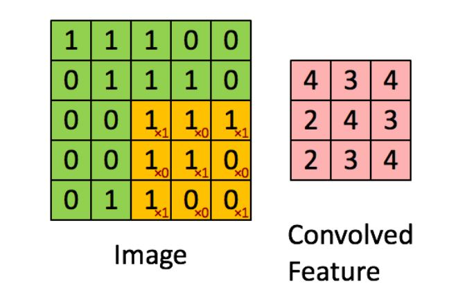
In this image, the green section shows the 5 x 5 x 1 formula. The yellow box evolves from the first box till last, performing the convolutional operation on every 3x3 matrix. This operation is called Kernel (K) and work on the basis of the following binary algorithm.


In the above figure, the Kernel moves to the right with a defined value for “Stride.” Along the way, it parses the image objects until it completes the breadth. Then it hops down to the second row on the left and moves just as in the top row till it covers the whole image. The process keeps repeating until every part of the image is parsed.
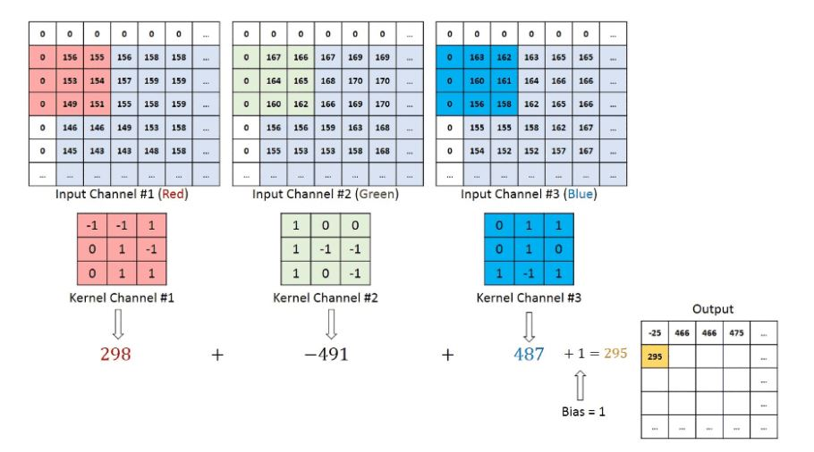
If there are multiple channels such as found in RGB images, then the kernel contains the same depth as found in the input image. The multiplication of the matrix is implemented based on the number of Ks. The procedure is followed as in stack format, for example, {K1, I1}, {K2, I2}, and so on. The results are generated based on the summation of bias. The result is in the form of a squeezed “1-depth channel” of convoluted feature output.
The goal of this convolution operation is to obtain all the high-level features of the image. The high-level features can include edges of the image too. This layer is not just limited to high-level features; it also performs an operation on low-level features, such as color and gradient orientation. This architecture evolves to a new level and thus includes two more types of layers. The two layers are known as Valid padding and the Same padding.
The objective of these layers is to reduce the dimensionality of the image that is found in the original input image and to increase dimensionality or, in some cases, to leave it unchanged, depending on the required output. The same padding is applied to convolute the image to different dimensions of the matrix, while valid padding is applied when there is no need to change the dimension of the matrix.
Pooling layer:
As identical to the recognized layer “convolutional,” the foremost aim of the Pooling layer is essential to decrease the spatial size of the Convolved Feature. So, in short words, it works for decreasing the required computational power for the processing of data by the method of dimensionality reduction. Moreover, it is also beneficial for the extraction of the dominant features, which are basically rotational as well as positional invariant, so the maintenance of the process effectively is needed.
Types of Pooling:
There are mainly two different types of Pooling which are as follows:
Max Pooling: The Max Pooling basically provides the maximum value within the covered image by the Kernel.
Average Pooling: The Average Pooling provides and returns the average value within the covered image by the Kernel.
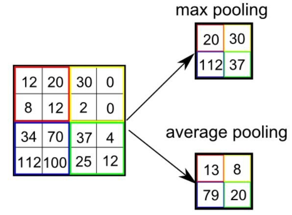
The other functionality of Max Pooling is also noise-suppressing, as it works on discarding those activations which contain noisy activation. And on the other side, the Average Pooling simply works on the mechanism of noise-suppressing by dimensionality reduction. So, in short words, we can conclude that Max Pooling works more efficiently than Average Pooling.
The Convolutional Layer, altogether with the Pooling layer, makes the “i-th layer” of the Convolutional Neural Network. Entirely reliant on the image intricacies, the layer counts might be rise-up for the objective of capturing the details of the detailed level, but also needs to have more computational power. After analyzing the above-described information about the process, we can easily execute the model for understanding the features. Moreover, here we are about to get the output and then provide it as an input for the regular Neural Network for further classification reasons.
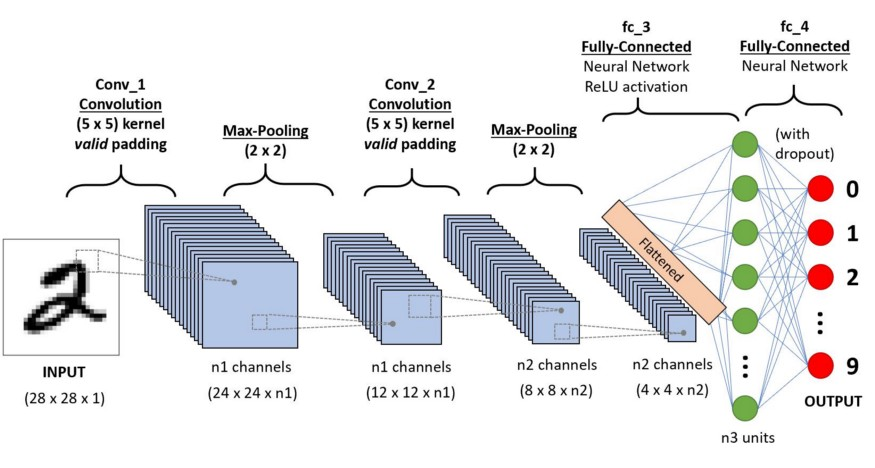
Classification: Fully Connected Layer (FC Layer)
The addition of the FC layer is mostly the easiest way for the learning purpose of the non-linear combinations of the abstract level structures, as it is also revealed by the output of the convolutional layer. The FC layer provides the space for learning non-linear functions. As now we have achieved our task to convert our image output into a specific form of Multi-layer Perceptron, now we must flatten the output image into a form of a column vector. Over the different eras of epochs, the model is basically succeeded for the distinguishing function between the dominating and low-level features.
Here are some impressive examples of CNN architectures:
- AlexNet
- GoogLeNet
- ZFNet
- LeNet
- ResNet
Summary:
In this article, the Convolutional Neural Network based on Deep Learning algorithm is explained. The workflow mechanism of CNN is explained with examples. The most powerful architectures in building CNN are given at the end which can help to make powerful AI algorithms for Computer Vision.
If you want to connect with me, please follow me on Twitter @bajcmartinez or visit my blog on computer science